TensorFlow - 循环神经网络

递归神经网络是一种面向深度学习的算法，它遵循顺序方法。 在神经网络中，我们总是假设每个输入和输出都独立于所有其他层。 这些类型的神经网络被称为循环神经网络，因为它们以顺序方式执行数学计算。

考虑以下步骤来训练循环神经网络 −

步骤 1 − 从数据集中输入特定示例。

步骤 2 − 网络将举一个例子，并使用随机初始化的变量计算一些计算。

步骤 3 − 然后计算预测结果。

步骤 4 − 生成的实际结果与期望值的比较会产生错误。

步骤 5 − 为了跟踪错误，它通过变量也被调整的相同路径传播。

步骤 6 − 重复从 1 到 5 的步骤，直到我们确信声明用于获取输出的变量已正确定义。

步骤 7 − 通过应用这些变量来获得新的看不见的输入，可以进行系统的预测。

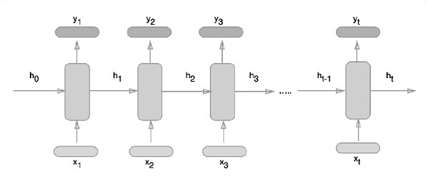
表示递归神经网络的示意图方法如下所述 −

使用 TensorFlow 实现循环神经网络

在本节中，我们将学习如何使用 TensorFlow 实现循环神经网络。

步骤 1 − TensorFlow 包括用于特定实现循环神经网络模块的各种库。

#Import necessary modules
from __future__ import print_function

import tensorflow as tf
from tensorflow.contrib import rnn
from tensorflow.examples.tutorials.mnist import input_data
mnist = input_data.read_data_sets("/tmp/data/", one_hot = True)

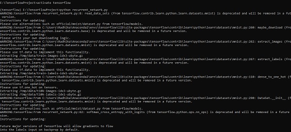
如上所述，这些库有助于定义输入数据，这是循环神经网络实现的主要部分。

步骤 2 − 我们的主要动机是使用循环神经网络对图像进行分类，我们将每个图像行视为一个像素序列。 MNIST 图像形状具体定义为 28*28 px。 现在我们将为提到的每个样本处理 28 个 28 个步骤的序列。 我们将定义输入参数以完成顺序模式。

n_input = 28 # MNIST data input with img shape 28*28
n_steps = 28
n_hidden = 128
n_classes = 10

# tf Graph input
x = tf.placeholder("float", [None, n_steps, n_input])
y = tf.placeholder("float", [None, n_classes]
weights = {
   'out': tf.Variable(tf.random_normal([n_hidden, n_classes]))
}
biases = {
   'out': tf.Variable(tf.random_normal([n_classes]))
}

步骤 3 − 使用 RNN 中定义的函数计算结果以获得最佳结果。 在这里，将每个数据形状与当前输入形状进行比较，并计算结果以保持准确率。

def RNN(x, weights, biases):
   x = tf.unstack(x, n_steps, 1)

   # Define a lstm cell with tensorflow
   lstm_cell = rnn.BasicLSTMCell(n_hidden, forget_bias=1.0)

   # Get lstm cell output
   outputs, states = rnn.static_rnn(lstm_cell, x, dtype = tf.float32)

   # Linear activation, using rnn inner loop last output
   return tf.matmul(outputs[-1], weights['out']) + biases['out']

pred = RNN(x, weights, biases)

# Define loss and optimizer
cost = tf.reduce_mean(tf.nn.softmax_cross_entropy_with_logits(logits = pred, labels = y))
optimizer = tf.train.AdamOptimizer(learning_rate = learning_rate).minimize(cost)

# Evaluate model
correct_pred = tf.equal(tf.argmax(pred,1), tf.argmax(y,1))
accuracy = tf.reduce_mean(tf.cast(correct_pred, tf.float32))

# Initializing the variables
init = tf.global_variables_initializer()

步骤 4 − 在这一步中，我们将启动图形以获取计算结果。 这也有助于计算测试结果的准确性。

with tf.Session() as sess:
   sess.run(init)
   step = 1
   # Keep training until reach max iterations
   
   while step * batch_size < training_iters:
      batch_x, batch_y = mnist.train.next_batch(batch_size)
      batch_x = batch_x.reshape((batch_size, n_steps, n_input))
      sess.run(optimizer, feed_dict={x: batch_x, y: batch_y})
      
      if step % display_step == 0:
         # Calculate batch accuracy
         acc = sess.run(accuracy, feed_dict={x: batch_x, y: batch_y})
         
         # Calculate batch loss
         loss = sess.run(cost, feed_dict={x: batch_x, y: batch_y})
         
         print("Iter " + str(step*batch_size) + ", Minibatch Loss= " + \
            "{:.6f}".format(loss) + ", Training Accuracy= " + \
            "{:.5f}".format(acc))
      step += 1
   print("Optimization Finished!")
      test_len = 128
   test_data = mnist.test.images[:test_len].reshape((-1, n_steps, n_input))
   
   test_label = mnist.test.labels[:test_len]
   print("Testing Accuracy:", \
      sess.run(accuracy, feed_dict={x: test_data, y: test_label}))

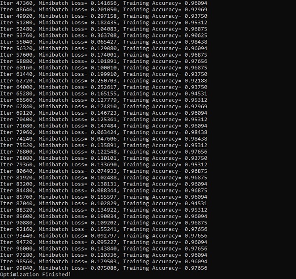
下面的屏幕截图显示了生成的输出 −