TensorFlow - 单层感知器

为了理解单层感知器，理解人工神经网络（ANN）很重要。 人工神经网络是一种信息处理系统，其机制受到生物神经回路功能的启发。 人工神经网络拥有许多相互连接的处理单元。 以下是人工神经网络的示意图 −

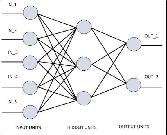
该图显示隐藏单元与外部层通信。 而输入和输出单元仅通过网络的隐藏层进行通信。

与节点的连接模式、输入和输出之间的总层数和节点级别以及每层神经元的数量定义了神经网络的架构。

有两种类型的架构。 这些类型侧重于功能性人工神经网络，如下所示 −

• 单层感知器
• 多层感知器

单层感知器

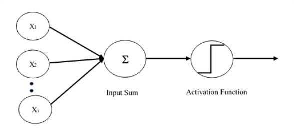
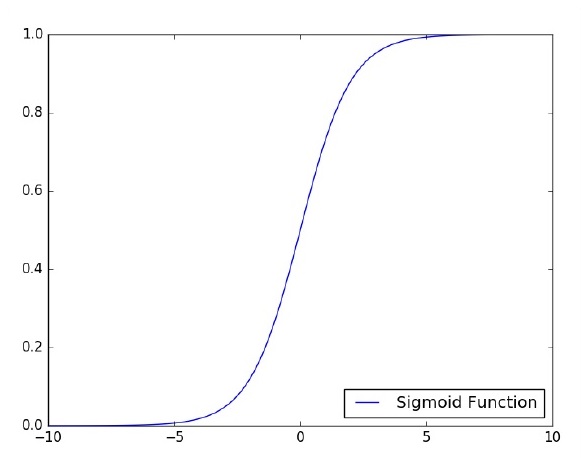
单层感知器是第一个提出的神经模型。 神经元的局部记忆内容由权重向量组成。 单层感知器的计算是通过计算输入向量的总和来执行的，每个向量的值乘以权重向量的对应元素。 输出中显示的值将是激活函数的输入。

让我们专注于使用 TensorFlow 实现图像分类问题的单层感知器。 说明单层感知器的最佳示例是通过"逻辑回归"的表示。

现在，让我们考虑以下训练逻辑回归的基本步骤 −

• 权重在训练开始时用随机值初始化。

• 对于训练集的每个元素，误差是根据期望输出与实际输出之间的差异来计算的。 计算出的误差用于调整权重。

• 重复这个过程，直到整个训练集的误差不小于指定的阈值，直到达到最大迭代次数。

下面提到了评估逻辑回归的完整代码 −

# Import MINST data 
from tensorflow.examples.tutorials.mnist import input_data 
mnist = input_data.read_data_sets("/tmp/data/", one_hot = True) 

import tensorflow as tf 
import matplotlib.pyplot as plt 

# Parameters 
learning_rate = 0.01 
training_epochs = 25 
batch_size = 100 
display_step = 1 

# tf Graph Input 
x = tf.placeholder("float", [None, 784]) # mnist data image of shape 28*28 = 784 
y = tf.placeholder("float", [None, 10]) # 0-9 digits recognition => 10 classes 

# Create model 
# Set model weights 
W = tf.Variable(tf.zeros([784, 10])) 
b = tf.Variable(tf.zeros([10])) 

# Construct model 
activation = tf.nn.softmax(tf.matmul(x, W) + b) # Softmax 

# Minimize error using cross entropy 
cross_entropy = y*tf.log(activation) 
cost = tf.reduce_mean\ (-tf.reduce_sum\ (cross_entropy,reduction_indices = 1)) 

optimizer = tf.train.\ GradientDescentOptimizer(learning_rate).minimize(cost) 

#Plot settings 
avg_set = [] 
epoch_set = [] 

# Initializing the variables init = tf.initialize_all_variables()
# Launch the graph 
with tf.Session() as sess:
   sess.run(init)
   
   # Training cycle
   for epoch in range(training_epochs):
      avg_cost = 0.
      total_batch = int(mnist.train.num_examples/batch_size)
      
      # Loop over all batches
      for i in range(total_batch):
         batch_xs, batch_ys = \ mnist.train.next_batch(batch_size)
         # Fit training using batch data sess.run(optimizer, \ feed_dict = {
            x: batch_xs, y: batch_ys}) 
         # Compute average loss avg_cost += sess.run(cost, \ feed_dict = {
            x: batch_xs, \ y: batch_ys})/total_batch
      # Display logs per epoch step
      if epoch % display_step == 0:
         print ("Epoch:", '%04d' % (epoch+1), "cost=", "{:.9f}".format(avg_cost))
            avg_set.append(avg_cost) epoch_set.append(epoch+1)
   print ("Training phase finished")
    
   plt.plot(epoch_set,avg_set, 'o', label = 'Logistic Regression Training phase') 
   plt.ylabel('cost') 
   plt.xlabel('epoch') 
   plt.legend() 
   plt.show() 
    
   # Test model 
   correct_prediction = tf.equal(tf.argmax(activation, 1), tf.argmax(y, 1)) 
   
   # Calculate accuracy 
   accuracy = tf.reduce_mean(tf.cast(correct_prediction, "float")) print 
      ("Model accuracy:", accuracy.eval({x: mnist.test.images, y: mnist.test.labels}))

输出

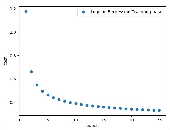
上面的代码生成以下输出 −

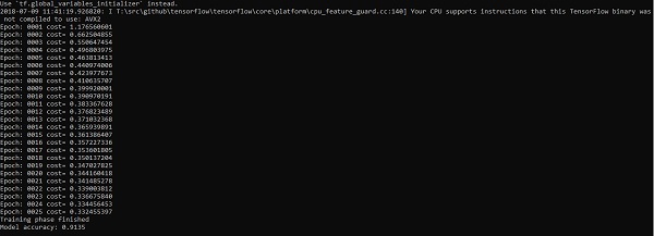
逻辑回归被认为是一种预测分析。 逻辑回归用于描述数据并解释一个因二元变量与一个或多个名义或自变量之间的关系。